Hidden Markov Models (HMMs) are a class of statistical models used to represent systems that follow a Markov process with hidden states. In such models, the system being modeled transitions between a finite number of states, with the probability of each transition dependent only on the current state. The hidden states are not directly observable; instead, we observe a sequence of emissions or outputs generated by these states. In other words these states emit different kinds of log returns with varying likelihood. One state might often emit very large log returns while another might emit very small returns.
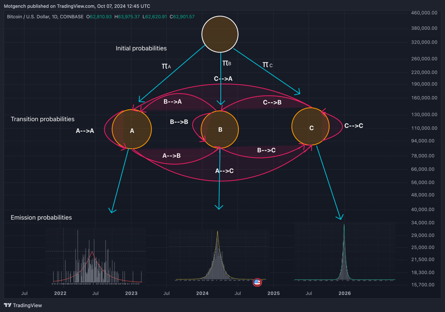
The log returns occurring in each state are modeled with a laplace distribution. In this way we can capture both the magnitude of returns often characterised as volatility as well as the expected value which often corresponds to the overall direction or drift present in the returns.
Beside the emission probabilities which explain how likely it is for an observation (log return) to have come from a specific state, the model is also governed by a transition matrix. The transition probabilities add an additional layer of information for the model to take into account. They inform the model how likely it is for a specific state to end and transition to any of the other states in the model. In plain words this means that the model is aware that if we are in an extremely volatile state it is most likely we transition to a less volatile state in the future, however perhaps not immediately to the most extreme low volatility state. The specifics can depend significantly on the exact architecture of the HMM as well as the number of states in the model.
This brings us to a slightly more advanced model, called the Hierarchical Hidden Markov Model. While HMMs model systems with a single layer of hidden states, each transitioning to other states based on fixed probabilities, HHMMs introduce multiple layers of hidden states.
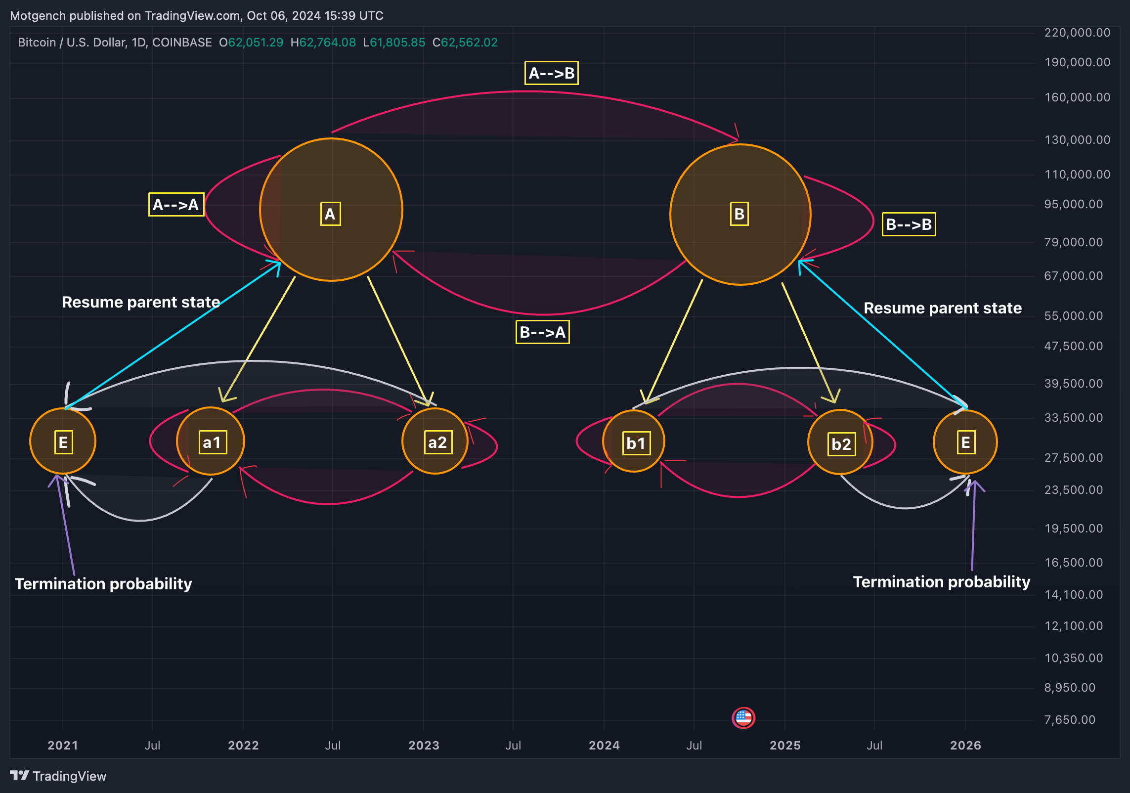
Multiple layers allow the model to capture longer term dependencies as well as more efficiently organise a larger number of states in the model. The HHMM depicted above comprises of 4 distinct states at the lowest lever of the hierarchy (a1,a2,b1,b2). The states in the lowest level of the hierarchy are called the production states, as they are the only states that generate/emit observations in our model.
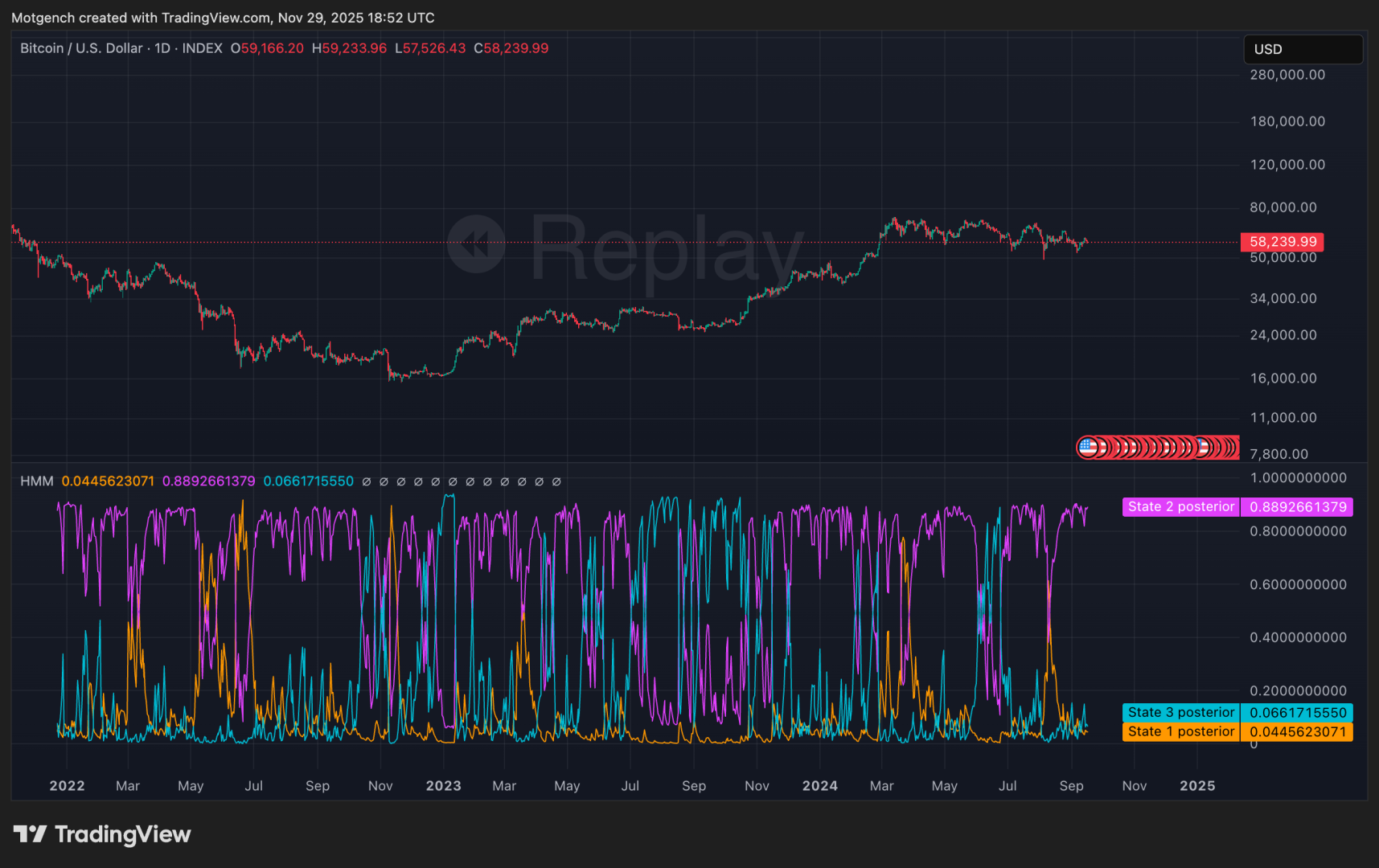
The different states identified by the model are often also called market regimes. A market regime is characterised by a specific persistent behaviour. As described before this could be either a period of high volatility, low volatility, uptrend or a downtrend. The indicator specifies the likelihood of being in a particular state at a given time through what we call the posterior probabilities.
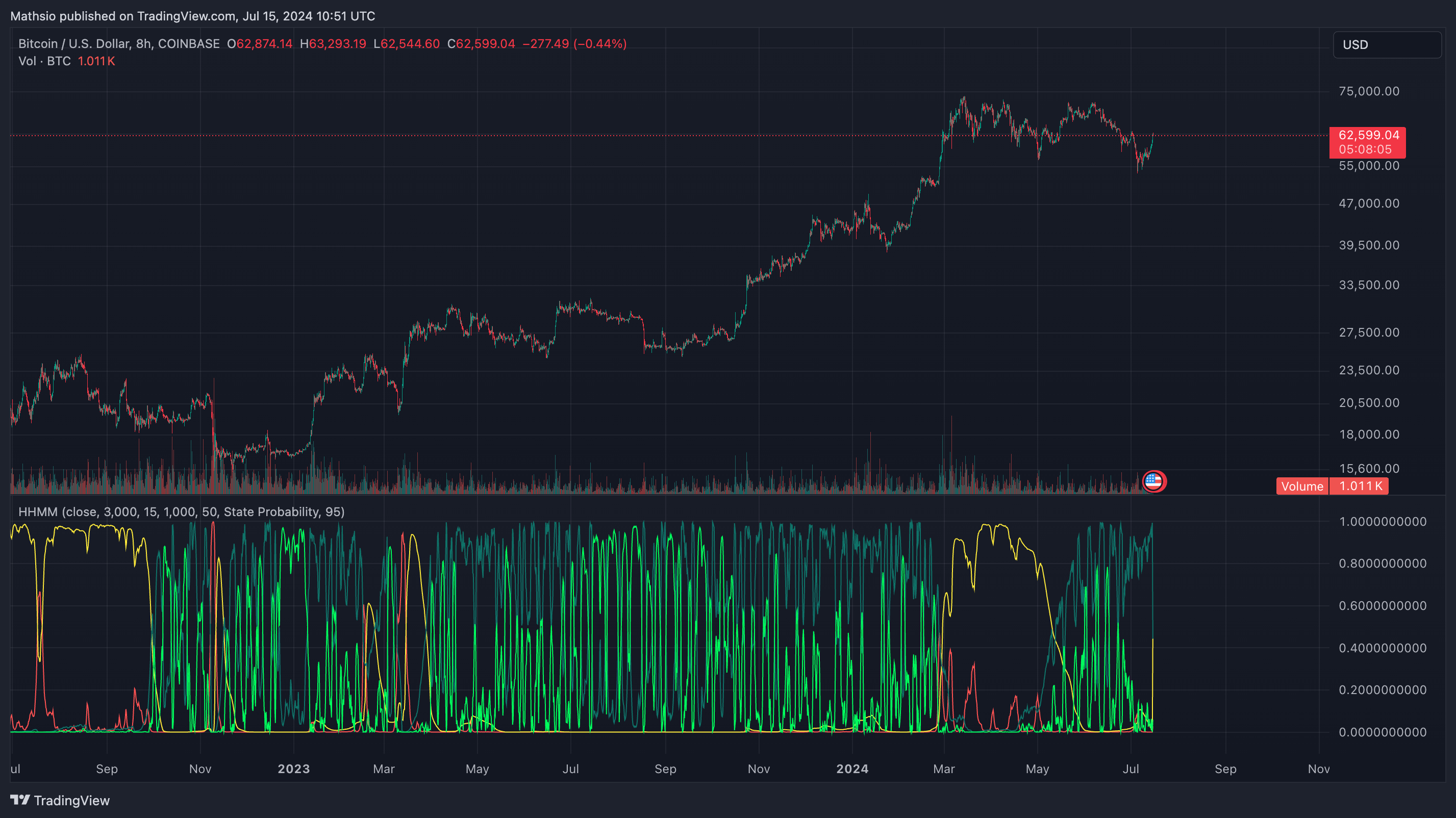
In this image we can see the posterior probabilities of each of the 4 production states in a HHMM. Each of the 4 coloured lines corresponds to a state in the model and the value at which any of the lines is specifies the probability of being in a particular hidden state or regime at a specific time given the data the model was trained on.
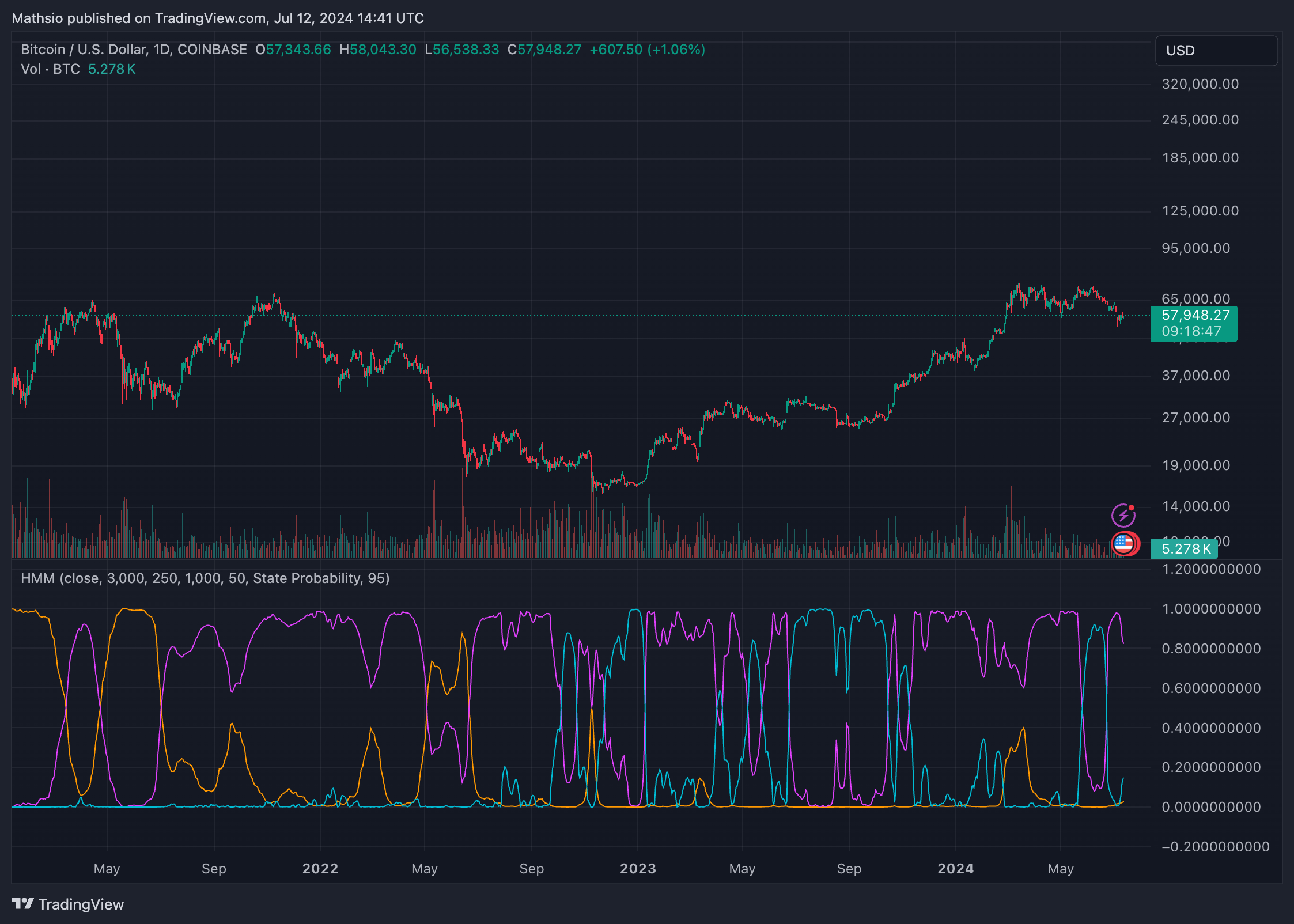
The same is done for a 3 state HMM as depicted below
Fitting the model as described above is just the first step in using Hidden Markov Models for analysis. Once the model is fitted we can use it to make out of sample predictions. Read more on in sample vs out of sample testing here
We can simply try to predict what state the market will be at the next time point as we do below:
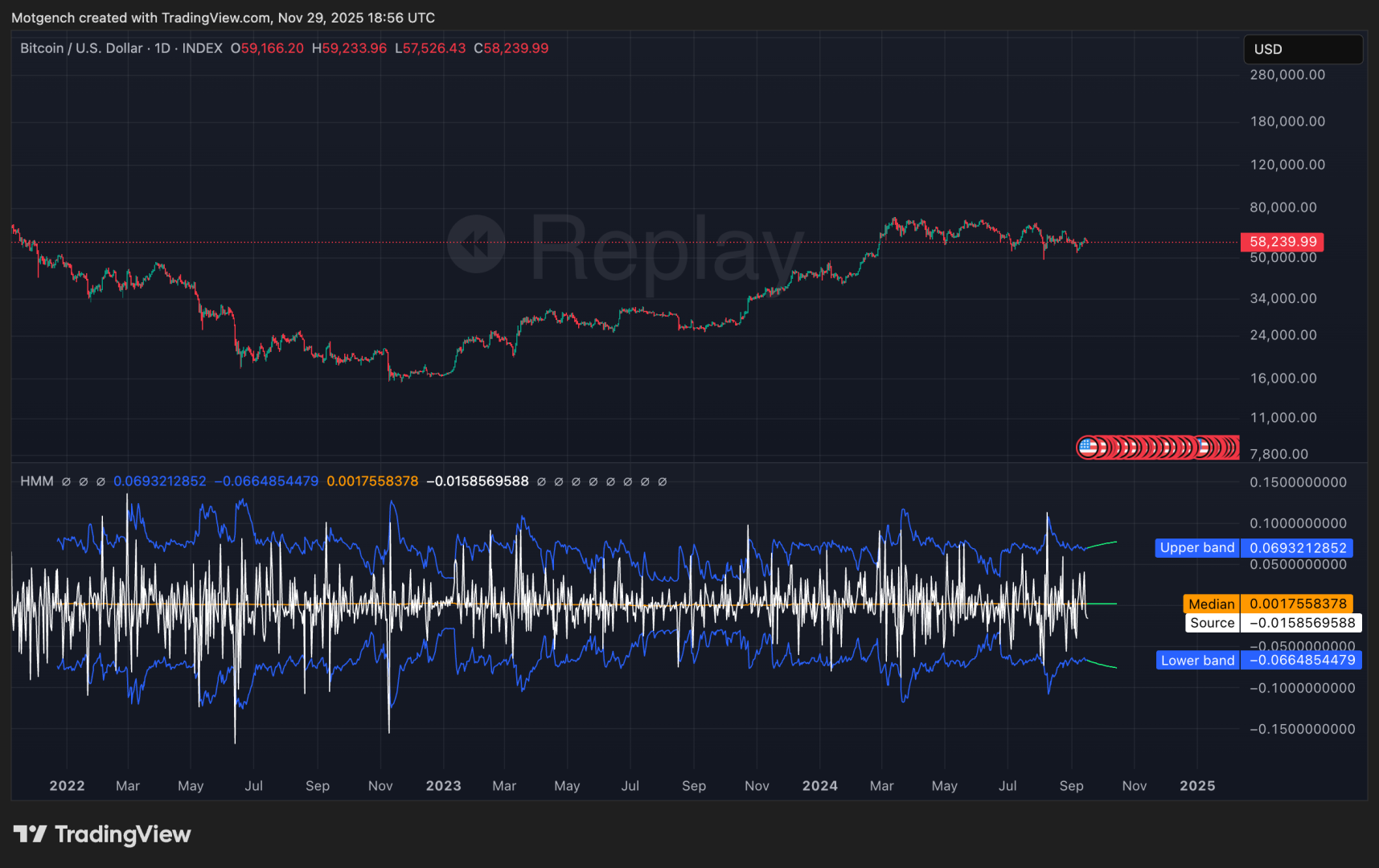
We can also construct confidence intervals for the next predicted datapoint.
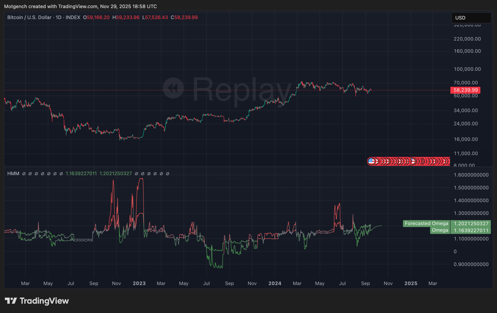
Or we can compute market state dependent risk adjusted metrics like sharpe ratio or in our case the omega ratio:
And for the last and my favourite use case, we can use Hidden Markov Models for generating state dependent probabilistic forecasts of future price movements via the Probability Cone:
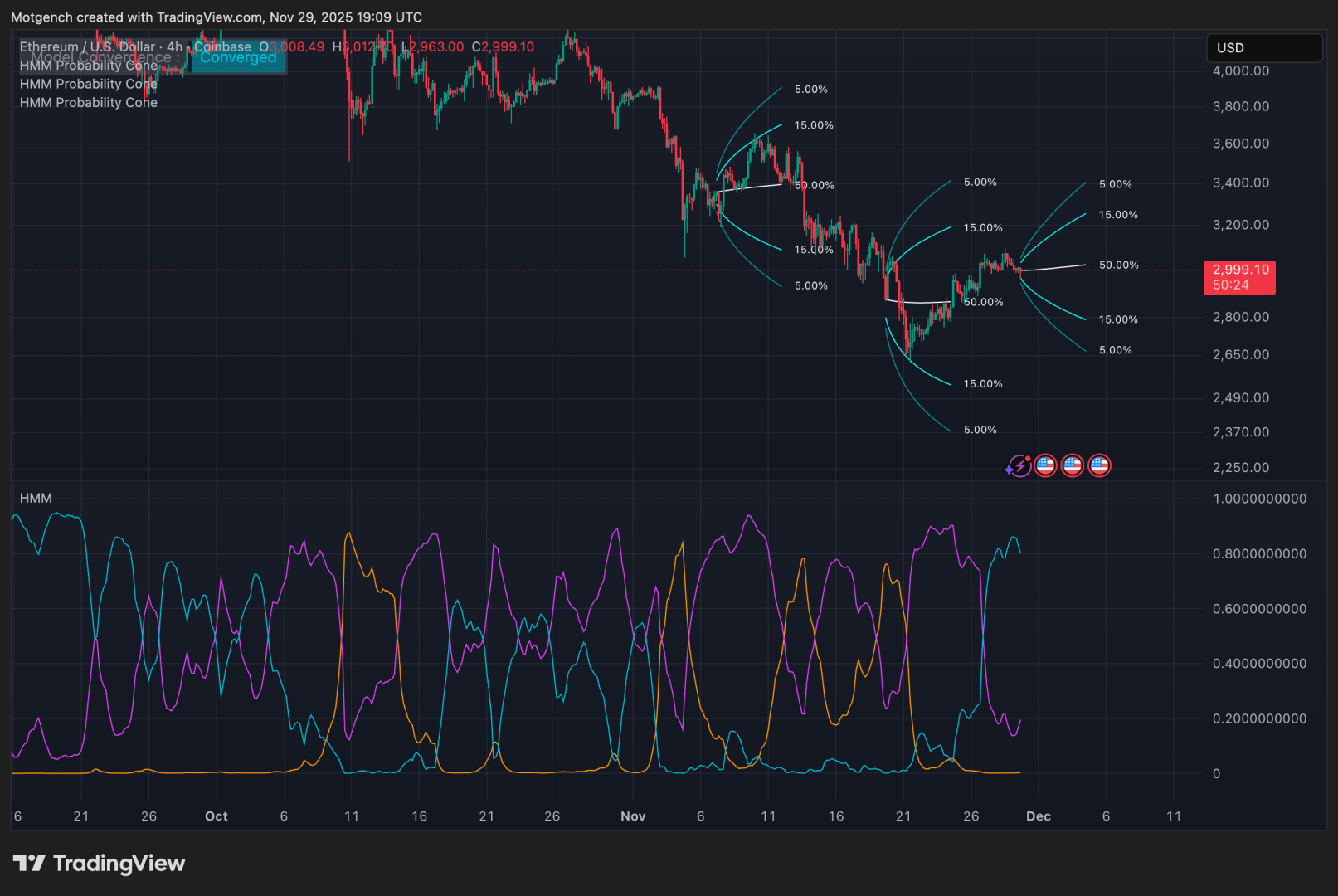
The state dependent probability cone is the full visual depiction of the models current expectation about the future price movements, based on the currently observed data, the current state and the most likely future transitions between states.
Below you can find more information on the Hidden Markov Model indicators:
Hidden Markov Model – Probability Cone